Level and plasticity divergence in a common trans-regulatory environment
source("functions_for_figure_scripts.R")
library(ggExtra)
load("data_files/FinalDataframe3Disp.RData")
load("data_files/Cleaned_Counts.RData")
load("data_files/Cleaned_Counts_Allele.RData")

cor_thresh <- 0.8
eff_thresh <- log2(1.5)
# extreme cor and log2 fold change values to extract the most
# cis plasticity divergers and most trans level divergers for
# avg expression figures
cis_dyn_thresh <- -0.25
trans_lev_thresh <- log2(2)
Log2 fold changes between parents and hybrid are correlated
# R squared for effect sizes between parents and hybrid for all genes
mod_full <- lm(effect_size_allele ~ effect_size_species, data = finaldf)
summary(mod_full)
##
## Call:
## lm(formula = effect_size_allele ~ effect_size_species, data = finaldf)
##
## Residuals:
## Min 1Q Median 3Q Max
## -18.053 -0.288 0.002 0.289 36.082
##
## Coefficients:
## Estimate Std. Error t value
## (Intercept) -0.085010 0.005148 -16.51
## effect_size_species 0.618360 0.004284 144.33
## Pr(>|t|)
## (Intercept) <2e-16 ***
## effect_size_species <2e-16 ***
## ---
## Signif. codes:
## 0 '***' 0.001 '**' 0.01 '*' 0.05 '.' 0.1 ' ' 1
##
## Residual standard error: 0.816 on 25254 degrees of freedom
## Multiple R-squared: 0.452, Adjusted R-squared: 0.452
## F-statistic: 2.083e+04 on 1 and 25254 DF, p-value: < 2.2e-16# R squared genes with consistent effect size and diverged level in at least one environment
levdiv_genes <- filter(finaldf, level == "diverged") |>
select(gene_name) |> pull() |> unique()
plotdf <- finaldf |> filter(gene_name %in% levdiv_genes) |>
group_by(gene_name) |> summarise(n_lev_dir = length(sign(effect_size_species))) |>
filter(n_lev_dir == 1)
mod <- lm(effect_size_allele ~ effect_size_species, data = filter(finaldf, gene_name %in% plotdf$gene_name))
summary(mod) # more correlated for genes with the most consistent level divergence across envrironments##
## Call:
## lm(formula = effect_size_allele ~ effect_size_species, data = filter(finaldf,
## gene_name %in% plotdf$gene_name))
##
## Residuals:
## Min 1Q Median 3Q Max
## -2.7550 -0.5028 0.0341 0.4596 3.8635
##
## Coefficients:
## Estimate Std. Error t value Pr(>|t|)
## (Intercept) -0.2588 0.1270 -2.038 0.0453
## effect_size_species 0.5236 0.0440 11.899 <2e-16
##
## (Intercept) *
## effect_size_species ***
## ---
## Signif. codes:
## 0 '***' 0.001 '**' 0.01 '*' 0.05 '.' 0.1 ' ' 1
##
## Residual standard error: 1.075 on 70 degrees of freedom
## Multiple R-squared: 0.6692, Adjusted R-squared: 0.6645
## F-statistic: 141.6 on 1 and 70 DF, p-value: < 2.2e-16# looping through each experiment
library(ggExtra)
plotlist <- vector(mode = "list", length = length(ExperimentNames))
names(plotlist) <- ExperimentNames
for (e in ExperimentNames) {
plotdf <- finaldf |> filter(experiment == e & level == "diverged")
mod_e <- lm(effect_size_allele ~ effect_size_species, data = plotdf)
plotlist[[e]] <- ggMarginal(ggplot(plotdf, aes(x = effect_size_species,
y = effect_size_allele)) +
geom_vline(xintercept = 0, alpha = 0.5) +
geom_hline(yintercept = 0, alpha = 0.5) +
geom_abline(slope = 1, intercept = 0, alpha = 0.5) +
geom_point(aes(color = experiment)) +
geom_text(x = -2, y = 4.5,
label = paste0("R^2 = ", round(summary(mod_e)$r.squared,
digits = 3))) +
scale_color_discrete(limits = colordf[colordf$scheme == "experiment",]$limits,
type = colordf[colordf$scheme == "experiment",]$type) +
xlim(c(-5, 5)) +
ylim(c(-5, 5)) +
xlab("") +
ylab("") +
ggtitle(LongExperimentNames[which(ExperimentNames == e)]) +
theme_classic() +
theme(legend.position = "none"),
groupColour = TRUE, groupFill = TRUE)
}## Warning: Removed 8 rows containing missing values or values
## outside the scale range (`geom_point()`).
## Removed 8 rows containing missing values or values
## outside the scale range (`geom_point()`).## Warning: Removed 4 rows containing missing values or values
## outside the scale range (`geom_point()`).
## Removed 4 rows containing missing values or values
## outside the scale range (`geom_point()`).## Warning: Removed 3 rows containing missing values or values
## outside the scale range (`geom_point()`).
## Removed 3 rows containing missing values or values
## outside the scale range (`geom_point()`).## Warning: Removed 1 row containing missing values or values
## outside the scale range (`geom_point()`).
## Removed 1 row containing missing values or values
## outside the scale range (`geom_point()`).## Warning: Removed 10 rows containing missing values or values
## outside the scale range (`geom_point()`).
## Removed 10 rows containing missing values or values
## outside the scale range (`geom_point()`).## Warning: Removed 12 rows containing missing values or values
## outside the scale range (`geom_point()`).
## Removed 12 rows containing missing values or values
## outside the scale range (`geom_point()`).pdf("paper_figures/CisTrans/l2fc_eachEnvironment.pdf",
width = 5, height = 8)
ggarrange(plotlist = plotlist, nrow = 3, ncol = 2)
dev.off()## quartz_off_screen
## 2ggarrange(plotlist = plotlist, nrow = 3, ncol = 2)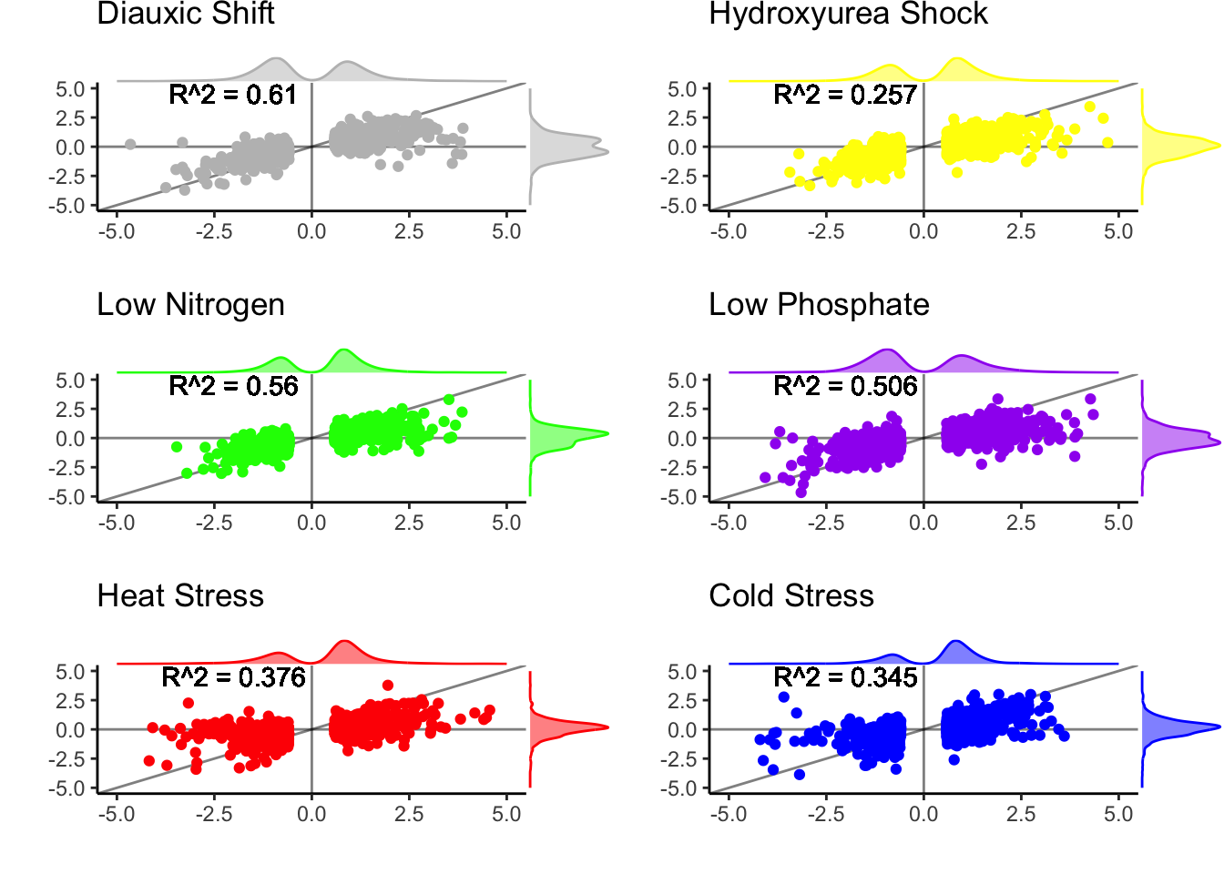
Hybrids have more correlated plasticity between alleles than parental orthologs
#### Distribution of parent/hybrid expression correlation ####
plotlist <- vector(mode = "list", length = length(ExperimentNames))
names(plotlist) <- ExperimentNames
# density plots of parental vs hybrid cor in each environment
for (e in ExperimentNames) {
  plotdf <- finaldf |> filter(experiment == e & plasticity == "diverged") |>
    select(gene_name, experiment, cor_parents, cor_hybrid) |>
    pivot_longer(cols = c("cor_parents", "cor_hybrid"),
                 names_to = "parent_or_hybrid",
                 values_to = "cor")
  plotlist[[e]] <- ggplot(plotdf, aes(x = cor)) +
    geom_density(data = filter(plotdf, parent_or_hybrid == "cor_parents"),
                 aes(fill = experiment), alpha = 1, color = "white") +
    geom_density(data = filter(plotdf, parent_or_hybrid == "cor_hybrid"),
                 aes(fill = experiment), alpha = 0.5, color = "black") +
    scale_fill_discrete(limits = colordf[colordf$scheme == "experiment",]$limits,
                        type = colordf[colordf$scheme == "experiment",]$type) +
    xlim(c(-1, 1)) +
    xlab("") +
    ylab("") +
    ggtitle(LongExperimentNames[which(ExperimentNames == e)]) +
    theme_classic() +
    theme(legend.position = "none")
}
p_null <- ggplot(plotdf) + theme_void()
pdf("paper_figures/CisTrans/cor_eachEnvironment.pdf",
    width = 8, height = 4)
ggarrange(plotlist[[1]], plotlist[[2]],
          p_null, p_null, plotlist[[3]], plotlist[[4]],
          plotlist[[5]], plotlist[[6]], nrow = 2, ncol = 4)
## Warning: Removed 2 rows containing non-finite outside the scale
## range (`stat_density()`).## Warning: Removed 1 row containing non-finite outside the scale
## range (`stat_density()`).
## Removed 1 row containing non-finite outside the scale
## range (`stat_density()`).
## Removed 1 row containing non-finite outside the scale
## range (`stat_density()`).
## Removed 1 row containing non-finite outside the scale
## range (`stat_density()`).
## Removed 1 row containing non-finite outside the scale
## range (`stat_density()`).## Warning: Removed 2 rows containing non-finite outside the scale
## range (`stat_density()`).
## Removed 2 rows containing non-finite outside the scale
## range (`stat_density()`).## Warning: Removed 1 row containing non-finite outside the scale
## range (`stat_density()`).
## Removed 1 row containing non-finite outside the scale
## range (`stat_density()`).
## Removed 1 row containing non-finite outside the scale
## range (`stat_density()`).dev.off()## quartz_off_screen
## 2ggarrange(plotlist[[1]], plotlist[[2]],
p_null, p_null, plotlist[[3]], plotlist[[4]],
plotlist[[5]], plotlist[[6]], nrow = 2, ncol = 4)## Warning: Removed 2 rows containing non-finite outside the scale
## range (`stat_density()`).
## Removed 1 row containing non-finite outside the scale
## range (`stat_density()`).
## Removed 1 row containing non-finite outside the scale
## range (`stat_density()`).
## Removed 1 row containing non-finite outside the scale
## range (`stat_density()`).
## Removed 1 row containing non-finite outside the scale
## range (`stat_density()`).
## Removed 1 row containing non-finite outside the scale
## range (`stat_density()`).## Warning: Removed 2 rows containing non-finite outside the scale
## range (`stat_density()`).
## Removed 2 rows containing non-finite outside the scale
## range (`stat_density()`).## Warning: Removed 1 row containing non-finite outside the scale
## range (`stat_density()`).
## Removed 1 row containing non-finite outside the scale
## range (`stat_density()`).
## Removed 1 row containing non-finite outside the scale
## range (`stat_density()`).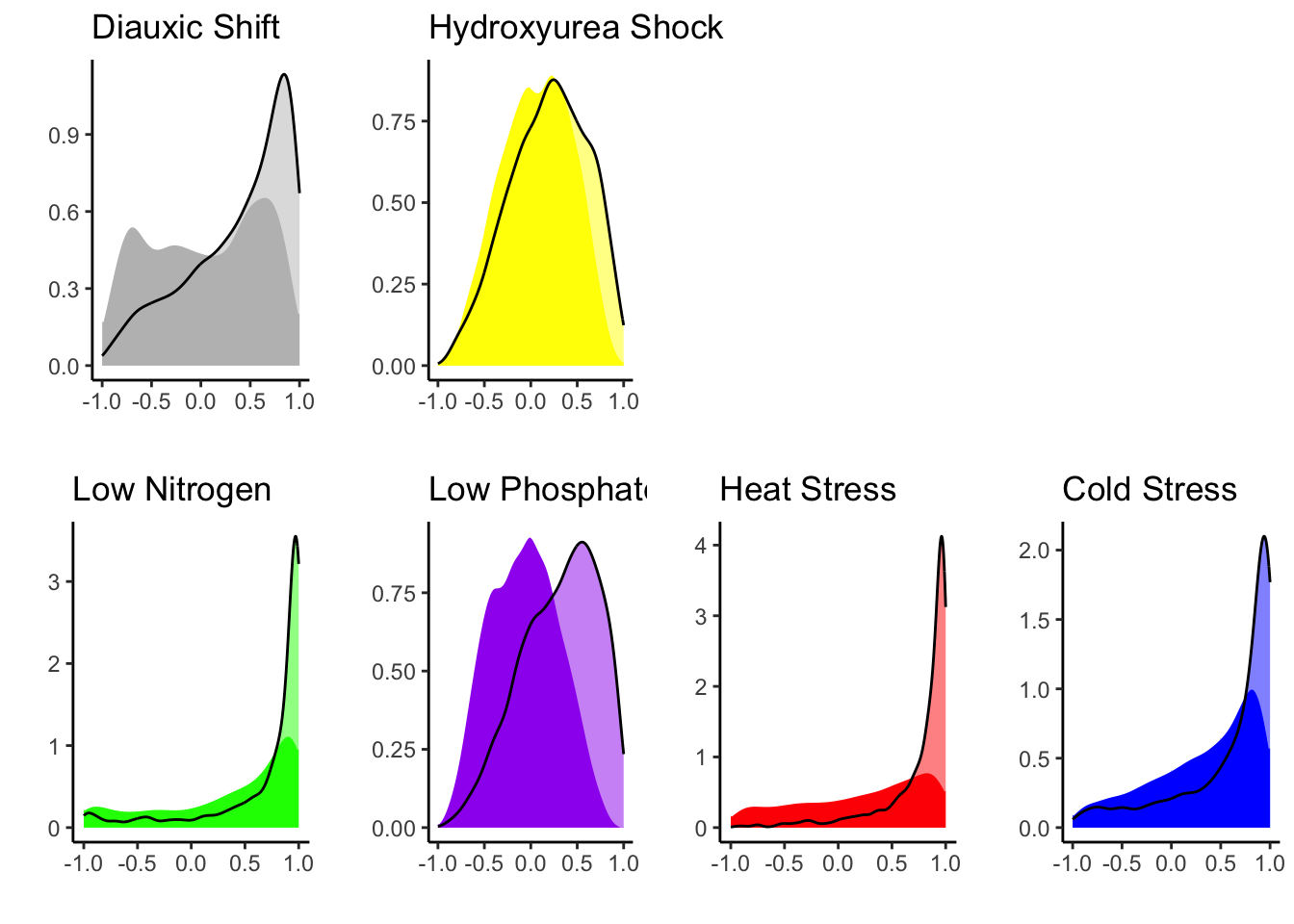
Level divergence tends to be in cis
What better way to show this than that looking at the small fraction of genes that are diverging in level in trans the most—that are diverging in level in the parents and have the smallest log2 fold change between hybrid alleles.
# pct genes in "transest level" group for figure
plotdf <- finaldf |>
  filter(level == "diverged") |>
  mutate(is_trans_upcer = (effect_size_species > trans_lev_thresh) &
           (abs(effect_size_allele) < eff_thresh),
         is_trans_uppar = (effect_size_species < -trans_lev_thresh) &
           (abs(effect_size_allele) < eff_thresh))
plotdf |> mutate(is_trans = is_trans_upcer | is_trans_uppar) |>
  group_by(experiment) |>
  summarise(pct_trans = sum(is_trans)/n(),
            pct_rest = sum(!is_trans)/n())
## # A tibble: 6 × 3
## experiment pct_trans pct_rest
## <chr> <dbl> <dbl>
## 1 CC 0.173 0.827
## 2 Cold 0.221 0.779
## 3 HAP4 0.148 0.852
## 4 Heat 0.236 0.764
## 5 LowN 0.135 0.865
## 6 LowPi 0.242 0.758pctdf <- plotdf |> mutate(is_trans = is_trans_upcer | is_trans_uppar) |>
group_by(experiment) |>
summarise(trans = sum(is_trans)/n(),
cis = sum(!is_trans)/n()) |>
pivot_longer(cols = c("cis", "trans"), names_to = "mode",
values_to = "percent")
p <- ggplot(pctdf, aes(x="", y=percent, fill=mode)) +
scale_fill_discrete(limits = c("cis", "trans"),
type = c("salmon", "aquamarine")) +
geom_bar(stat="identity", width=1) +
coord_polar("y", start=0) +
theme_classic() +
theme(axis.ticks = element_blank(),
axis.text = element_blank(),
legend.position = "bottom") +
xlab("") +
ylab("") +
facet_wrap(~factor(experiment, levels = ExperimentNames,
labels = LongExperimentNames), nrow = 2, ncol = 3)
pdf("paper_figures/CisTrans/level_pcts.pdf",
width = 8, height = 4)
p
dev.off()## quartz_off_screen
## 2p
Average expression of the cis and trans portion of level divergers, Diauxic Shift as example:
plotdf <- finaldf |>
  filter(level == "diverged") |>
  mutate(is_trans_upcer = (effect_size_species > trans_lev_thresh) &
           (abs(effect_size_allele) < eff_thresh),
         is_trans_uppar = (effect_size_species < -trans_lev_thresh) &
           (abs(effect_size_allele) < eff_thresh))
plotdf |> mutate(is_trans = is_trans_upcer | is_trans_uppar) |>
  group_by(experiment) |>
  summarise(pct_trans = sum(is_trans)/n(),
            pct_rest = sum(!is_trans)/n())
## # A tibble: 6 × 3
## experiment pct_trans pct_rest
## <chr> <dbl> <dbl>
## 1 CC 0.173 0.827
## 2 Cold 0.221 0.779
## 3 HAP4 0.148 0.852
## 4 Heat 0.236 0.764
## 5 LowN 0.135 0.865
## 6 LowPi 0.242 0.758# upcer, trans
gene_idxs <- filter(plotdf, experiment == "HAP4" & cer == 1 &
par == 1 & is_trans_upcer) |>
select(gene_name) |> pull()
p <- annotate_figure(plotGenes(gene_idxs, .quartet = TRUE,
.experiment_name = "HAP4"),
top = paste(length(gene_idxs), "genes"))## `summarise()` has grouped output by 'group_id',
## 'gene_name', 'experiment'. You can override using the
## `.groups` argument.
## `summarise()` has grouped output by 'time_point_num',
## 'experiment'. You can override using the `.groups`
## argument.
## Adding missing grouping variables: `time_point_num`,
## `experiment`
## Adding missing grouping variables: `time_point_num`,
## `experiment`p
pdf("paper_figures/CisTrans/level_trans_HAP411_upcer.pdf", width = 3, height = 3)
p
dev.off()
## quartz_off_screen
## 2# upcer, cis
gene_idxs <- filter(plotdf, experiment == "HAP4" & cer == 1 &
par == 1 & !is_trans_upcer & !is_trans_uppar &
effect_size_species > 0) |>
select(gene_name) |> pull()
p <- annotate_figure(plotGenes(gene_idxs, .quartet = TRUE,
.experiment_name = "HAP4"),
top = paste(length(gene_idxs), "genes"))## `summarise()` has grouped output by 'group_id',
## 'gene_name', 'experiment'. You can override using the
## `.groups` argument.
## `summarise()` has grouped output by 'time_point_num',
## 'experiment'. You can override using the `.groups`
## argument.
## Adding missing grouping variables: `time_point_num`,
## `experiment`
## Adding missing grouping variables: `time_point_num`,
## `experiment`p
pdf("paper_figures/CisTrans/level_cis_HAP411_upcer.pdf", width = 3, height = 3)
p
dev.off()
## quartz_off_screen
## 2Plasticity divergence tends to be in trans
plotdf <- finaldf |>
  filter(plasticity == "diverged") |>
  mutate(is_cis = cor_hybrid < cis_dyn_thresh)
plotdf |> group_by(experiment) |>
  summarise(cis = sum(is_cis, na.rm = TRUE)/n(),
            trans = sum(!is_cis, na.rm = TRUE)/n())
## # A tibble: 6 × 3
## experiment cis trans
## <chr> <dbl> <dbl>
## 1 CC 0.161 0.838
## 2 Cold 0.103 0.896
## 3 HAP4 0.148 0.852
## 4 Heat 0.0321 0.967
## 5 LowN 0.0858 0.913
## 6 LowPi 0.105 0.893pctdf <- plotdf |> group_by(experiment) |>
summarise(cis = sum(is_cis, na.rm = TRUE)/n(),
trans = sum(!is_cis, na.rm = TRUE)/n()) |>
pivot_longer(cols = c("cis", "trans"), names_to = "mode",
values_to = "percent")
p <- ggplot(pctdf, aes(x="", y=percent, fill=mode)) +
scale_fill_discrete(limits = c("cis", "trans"),
type = c("salmon", "aquamarine")) +
geom_bar(stat="identity", width=1) +
coord_polar("y", start=0) +
theme_classic() +
theme(axis.ticks = element_blank(),
axis.text = element_blank(),
legend.position = "bottom") +
xlab("") +
ylab("") +
facet_wrap(~factor(experiment, levels = ExperimentNames,
labels = LongExperimentNames), nrow = 2, ncol = 3)
p
pdf("paper_figures/CisTrans/plasticity_pcts.pdf",
    width = 8, height = 4)
p
dev.off()
## quartz_off_screen
## 2Average expression of Diauxic Shift example:
plotdf <- finaldf |>
  filter(plasticity == "diverged") |>
  mutate(is_cis = cor_hybrid < cis_dyn_thresh)
plotdf |> group_by(experiment) |>
  summarise(cis = sum(is_cis, na.rm = TRUE)/n(),
            trans = sum(!is_cis, na.rm = TRUE)/n())
## # A tibble: 6 × 3
## experiment cis trans
## <chr> <dbl> <dbl>
## 1 CC 0.161 0.838
## 2 Cold 0.103 0.896
## 3 HAP4 0.148 0.852
## 4 Heat 0.0321 0.967
## 5 LowN 0.0858 0.913
## 6 LowPi 0.105 0.893# cis
gene_idxs <- filter(plotdf, experiment == "HAP4" & cer == 2 &
par == 1 & is_cis) |>
select(gene_name) |> pull()
p <- annotate_figure(plotGenes(gene_idxs, .quartet = TRUE,
.experiment_name = "HAP4"),
top = paste(length(gene_idxs), "genes"))## `summarise()` has grouped output by 'group_id',
## 'gene_name', 'experiment'. You can override using the
## `.groups` argument.
## `summarise()` has grouped output by 'time_point_num',
## 'experiment'. You can override using the `.groups`
## argument.
## Adding missing grouping variables: `time_point_num`,
## `experiment`
## Adding missing grouping variables: `time_point_num`,
## `experiment`p
pdf("paper_figures/CisTrans/plasticity_cis_HAP421.pdf",
        width = 3, height = 3)
p
dev.off()
## quartz_off_screen
## 2# trans
gene_idxs <- filter(plotdf, experiment == "HAP4" & cer == 2 &
par == 1 & !is_cis) |>
select(gene_name) |> pull()
p <- annotate_figure(plotGenes(gene_idxs, .quartet = TRUE,
.experiment_name = "HAP4"),
top = paste(length(gene_idxs), "genes"))## `summarise()` has grouped output by 'group_id',
## 'gene_name', 'experiment'. You can override using the
## `.groups` argument.
## `summarise()` has grouped output by 'time_point_num',
## 'experiment'. You can override using the `.groups`
## argument.
## Adding missing grouping variables: `time_point_num`,
## `experiment`
## Adding missing grouping variables: `time_point_num`,
## `experiment`p
pdf("paper_figures/CisTrans/plasticity_trans_HAP421.pdf",
        width = 3, height = 3)
p
dev.off()
## quartz_off_screen
## 2